Archive

Archives pour la catégorie ‘Réseau’

How to set up web-based network traffic monitoring system on Linux

23/11/2023 Comments off

When you are tasked with monitoring network traffic on the local network, you can consider many different options to do it, depending on the scale/traffic of the local network, monitoring platforms/interface, types of backend database, etc.

ntopng is an open-source (GPLv3) network traffic analyzer which provides a web interface for real-time network traffic monitoring. It runs on multiple platforms including Linux and MacOS X. ntopng comes with a simple RMON-like agent with built-in web server capability, and uses Redis-backed key-value server to store time series statistics. You can install ntopng network traffic analyzer on any designated monitoring server connected to your network, and use a web browser to access real-time traffic reports available on the server.

In this tutorial, I will describe how to set up a web-based network traffic monitoring system on Linux by using ntopng.

Features of ntopng

  • Flow-level, protocol-level real-time analysis of local network traffic.
  • Domain, AS (Autonomous System), VLAN level statistics.
  • Geolocation of IP addresses.
  • Deep packet inspection (DPI) based service discovery (e.g., Google, Facebook).
  • Historical traffic analysis (e.g., hourly, daily, weekly, monthly, yearly).
  • Support for sFlow, NetFlow (v5/v9) and IPFIX through nProbe.
  • Network traffic matrix (who’s talking to who?).
  • IPv6 support.

Install ntopng on Linux

The official website offers binary packages for Ubuntu and CentOS. So if you use either platform, you can install these packages.

If you want to build the latest ntopng from its source, follow the instructions below. (Update: these instructions are valid for ntopng 1.0. For ntopng 1.1 and higher, see the updated instructions).

To build ntopng on Debian, Ubuntu or Linux Mint:

$ sudo apt-get install libpcap-dev libglib2.0-dev libgeoip-dev redis-server wget libxml2-dev
$ tar xzf ntopng-1.0.tar.gz -C ~
$ cd ~/ntopng-1.0/
$ ./configure
$ make geoip
$ make

In the above steps, « make geoip » will automatically download a free version of GeoIP databases with wget from maxmind.com. So make sure that your system is connected to the network.

To build ntopng on Fedora:

$ sudo yum install libpcap-devel glib2-devel GeoIP-devel libxml2-devel libxml2-devel redis wget
$ tar xzf ntopng-1.0.tar.gz -C ~
$ cd ~/ntopng-1.0/
$ ./configure
$ make geoip
$ make

To install ntopng on CentOS or RHEL, first set up EPEL repository, and then follow the same instructions as in Fedora above.

Configure ntopng on Linux

After building ntopng, create a configuration directory for ntopng, and prepare default configuration files as follows. I assume that « 192.168.1.0/24 » is the CIDR address prefix of your local network.

$ sudo mkir /etc/ntopng -p
$ sudo -e /etc/ntopng/ntopng.start
--local-networks "192.168.1.0/24"
--interface 1
$ sudo -e /etc/ntopng/ntopng.conf
-G=/var/run/ntopng.pid

Lire la suite…

How to check Internet speed from the command line on Linux

22/11/2023 Comments off

check internet speedWhen you are experiencing slow Internet access, you may want to test the Internet speed of your upstream ISP (often called « last mile » in the residential broadband networks) as part of troubleshooting. For that matter, Speedtest.net is probably the most widely used broadband speed testing website.

Underneath it, Speedtest.net loads JavaScript code in your web browser, which then automatically detects the closest Speedtest.net server from you, and measures download/upload speed by sending HTTP GET and POST requests to the server.

However, if you are trying to check Internet speed from a remote headless server, VPS or an otherwise desktop-less system, Speedtest.net’s Flash-based user-friendly interface would be no good. For those of you, there is a command-line interface (CLI) version of Speedtest.net, known as speedtest-cli. Here I will demonstrate how to use speedtest-cli to check Internet speed from the command line in Linux.

Install speedtest-cli on Linux

speedtest-cli is a simple CLI client written in Python for measuring bidirectional Internet bandwidth by using Speedtest.net infrastructure. It works with Python 2.4-3.4. Installing the latest speedtest-cli is nothing more than downloading the Python script.

$ wget https://raw.github.com/sivel/speedtest-cli/master/speedtest_cli.py
$ chmod a rx speedtest_cli.py
$ sudo mv speedtest_cli.py /usr/local/bin/speedtest-cli
$ sudo chown root:root /usr/local/bin/speedtest-cli

Test Internet Connection Speed with speedtest-cli

It is straightforward to check your Internet speed with speedtest-cli. Running speedtest-cli command without any argument gets its job done.

$ speedtest-cli

This will automatically discover the closest Speedtest.net server (in terms of geographic distance), and report download and upload speed measured from the server.


If you want to share the speed test result, you can use « --share » option, which will allow you to share speed test result with others in an image format via Speedtest.net.

The following is a sample image automatically generated and uploaded to Speedtest.net by speedtest-cli.

Lire la suite…

Categories: Réseau Tags:

How to look up the geographic location of an IP address from the command line

22/11/2023 Comments off

geographic location ipIf you want to find out where a given IP address is physically located on earth, there are quite a few online GeoIP lookup services you can try (e.g. geoiptool.com). These online services are mostly powered by freely available GeoIP databases such as those from MaxMind. Besides using such web-based services, there are different ways to query the GeoIP databases, notably via the Linux command line.

In this tutorial, I am going to describe how to geolocate an IP address from the command line in Linux.

Method One

The first method is to use geoiplookup tool which is a command-line client for MaxMind’s GeoIP databases. geoiplookup allows you to look up the geography or network information of an IP address (or hostname). You can install the tool (along with the free GeoIP database used by the tool) as follows.

To install geoiplookup on Debian, Ubuntu or Linux Mint:

$ sudo apt-get install geoip-bin

To install geoiplookup on Fedora:

$ sudo yum install geoip

To install geoiplookup on CentOS, first enable EPEL repository, and then use yum command:

$ sudo yum install geoip

The default installation of geoiplookup comes with GeoIP.dat database file which is located in /usr/share/GeoIP. With this database, you can look up the country information only.

 
$ geoiplookup 23.66.166.151
GeoIP Country Edition: US, United States

You can download additional GeoIP databases from MaxMind, which give you more detailed information about IP addresses beyond country info. You can also download more up-to-date GeoIP.dat from the site. This is recommended because GeoIP.dat may have already been outdated by the time you install it from Linux repositories. The GeoIP databases available on MaxMind website are updated every month.

To install additional GeoIP databases from MaxMind, do the following. You may want to set up a monthly cronjob to automate this process.

$ wget http://geolite.maxmind.com/download/geoip/database/GeoLiteCountry/GeoIP.dat.gz
$ wget http://geolite.maxmind.com/download/geoip/database/GeoLiteCity.dat.gz
$ wget http://download.maxmind.com/download/geoip/database/asnum/GeoIPASNum.dat.gz
$ gunzip GeoIP.dat.gz
$ gunzip GeoIPASNum.dat.gz
$ gunzip GeoLiteCity.dat.gz
$ sudo cp GeoIP.dat GeoIPASNum.dat GeoLiteCity.dat /usr/share/GeoIP/

Now if you re-run geoiplookup, you will see the additional AS number information of an IP address. This basically tells you which administrative domain the IP address belongs to.

$ geoiplookup 128.112.119.209
GeoIP Country Edition: US, United States
GeoIP ASNum Edition: AS88 Princeton University

When run without any parameter, geoiplookup tool automatically uses GeoIP.dat and GeoIPASNum.dat only, but not use GeoLiteCity.dat. The latter can give you city-level information.

To obtain city-level geolocation information, explicitly tell geoiplookup to use GeoLiteCity.dat database.

$ geoiplookup -f /usr/share/GeoIP/GeoLiteCity.dat 23.66.166.151
GeoIP City Edition, Rev 1: US, MA, Cambridge, 02142, 42.362598, -71.084297, 506, 617

The output includes state, city, zipcode, latitude and longitude. The accuracy of the inferred location varies across different countries and networks. For example, the geolocation result tends to be more accurate for broadband IP addresses, but not as accurate for mobile networks.

Method Two

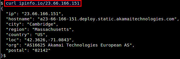
If you want to avoid the hassle of installing and updating GeoIP databases, you can try ipinfo.io online service. Unlike other services, ipinfo.io provides JSON-based geolocation API, so you can easily look up geolocation from the command line, using tools like curl.

$ curl ipinfo.io/23.66.166.151

13117907603_3cce4123de_z

Note that the access to their API is rate-limited at 1,000 API requests per day.

Source: Xmodulo

Change the IPTables log file

21/11/2023 Comments off

An important aspect of any firewall are the log files. Iptables on Linux provides logging functionality, however by default, it will get outputted to the /var/log/messages log file. This can clutter things up, and make it hard to check the logs.

If you want to change the file that IPTables logs to, you need to set up your iptables rules to output a log prefix. Rsyslog will then be configured to pick up this prefix, and output the information to a custom log file, containing just the iptables log information.
Install rsyslog if it is not already installed.

$ sudo apt-get install -y rsyslog

Lire la suite…

Categories: Réseau, Système Tags: , , ,

Voyage au centre du noyau: Traffic Control, la QoS

18/11/2023 Comments off

Gérer la QoS.

On peut aujourd’hui largement envisager d’héberger un ou plusieurs services sur son serveur à domicile, et des mouvements comme auto-hebergement.fr l’on bien illustré. Reste le problème de la bande passante en upload, qui bien que largement suffisante pour héberger des serveurs web, email, jabber ou autre, reste à utiliser intelligemment.

Linux fournit cette intelligence, sous forme d’un scheduler de paquets nommé Traffic Control (TC, pour les intimes), et l’objectif de cet article est de présenter cette technologie et sa mise en place dans un cas d’étude d’hébergement Web, DNS et même BitTorrent. Notons au passage que bon nombre de scripts et programmes existent pour simplifier la mise en place de la QoS (Quality of Service). Citons Wondershaper, Shorewall, ADSL-Optimizer par exemple. Cet article n’en parlera pas, car l’objectif est ici de faire mais aussi de comprendre comment ça marche sous le capot, et pour ça, il faut démonter le moteur et mettre les mains dans le cambouis.

1. Traffic Control, la QoS, les bases

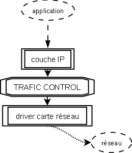
Traffic Control travaille sur les paquets sortant du noyau. Il n’a pas, initialement, pour objectif de contrôler le trafic des paquets entrants. Cette portion de code du noyau se situe entre la couche IP et le pilote du matériel qui transmet sur le réseau. On est donc très bas dans les couches. En réalité, c’est Traffic Control qui est constamment en charge de transmettre au driver de la carte réseau le paquet à envoyer.

figure1-tcgeneral

Cela signifie, en fait, que le module TC – le scheduler de paquet – est en permanence activé dans le noyau, même quand vous ne pensez pas l’utiliser. Par défaut, ce scheduler maintient une queue (prononcer kiou, une file d’attente) similaire à FIFO dans laquelle le premier paquet entré est donc le premier sortit.

La base de TC est la Queuing Discipline (qdisc) qui représente la politique de scheduling appliquée à une queue. Il existe différentes qdisc. Comme pour le scheduling processeur, on retrouve les méthodes FIFO, FIFO à plusieurs files, FIFO avec hash et round robin (SFQ). On a également un système Token Bucket Filter (TBF) qui attribue des jetons (tokens) à une qdisc pour en limiter le débit (pas de token = pas de transmission = on attend d’avoir un jeton disponible). Cette dernière politique a ensuite été étendue à un TBF hiérarchique, le HTB (Hierarchical Token Bucket). Les politiques que nous allons étudier ici sont TBF, qui pose les fondamentaux, SFQ et HTB. Nous allons également jeter un coup d’oeil à la politique par défaut, que, tout Monsieur Jourdain que nous sommes, nous utilisons sans le savoir: pfifo_fast.

1.1 Premier contact

Jean-Kevin est pressé, il n’a pas de temps à perdre, et tout de suite maintenant, il doit limiter la bande passante sortante de son serveur web à 200kbits par secondes (25ko/s). Au diable la théorie, on y reviendra plus tard, mettons tout de suite les mains dans le cambouis. La mécanique que nous allons mettre en place est simple. Nous allons utiliser une règle Netfilter pour marquer les paquets qui nous intéressent. Ensuite, nous allons fournir à TC une politique qui s’appliquera sur les paquets contenant la marque définie. C’est parti.

1.2 Netfilter MARK

Netfilter permet d’interagir directement avec la structure représentant un paquet dans le noyau. Cette structure, le sk_buff, possède un champ « __u32 nfmark » que l’on va renseigner et qui sera lu par le filtre de TC pour sélectionner la classe de destination du paquet. La règle iptables suivante va appliquer la marque ’80’ sur les paquets sortant (chaine OUTPUT) ayant pour port source le port 80:

# iptables -t mangle -A OUTPUT -o eth0 -p tcp --sport 80 -j MARK --set-mark 80

On peut vérifier que cette règle est bien appliquée aux paquets sortants en visualisant les statistiques de Netfilter.

# iptables -L OUTPUT -t mangle -v
Chain OUTPUT (policy ACCEPT 74107 packets, 109M bytes)
 pkts bytes target prot opt in  out  source   destination
73896  109M MARK   tcp  --  any eth0 anywhere anywhere    tcp spt:www MARK xset 0x50/0xffffffff

1.3 Deux classes dans un arbre

Le binaire /sbin/tc est compris dans le package iproute (sous Debian). Un simple aptitude suffit à l’installer, s’il ne l’est pas déjà. Nous allons créer un arbre dont la racine appliquera la politique HTB. Cet arbre va contenir deux classes: une pour notre trafic marqué, l’autre pour tout le reste et qui sera donc considérée par défaut.

# tc qdisc add dev eth0 root handle 1: htb default 20
# tc class add dev eth0 parent 1:0 classid 1:10 htb rate 200kbit ceil 200kbit prio 1 mtu 1500
# tc class add dev eth0 parent 1:0 classid 1:20 htb rate 1024kbit ceil 1024kbit prio 2 mtu 1500

Les deux classes filles sont raccrochés à la racine. Ces classes possèdent un débit garantie (rate) et un débit maximal opportuniste (ceil). Si la bande passante n’est pas utilisée, alors une classe pourra monter son débit jusqu’à la valeur de ceil. Sinon c’est la valeur de rate qui s’applique. Cela veut dire que la somme des valeurs de rate doit correspondre à la bande passante disponible. Dans le cas d’un upload ADSL classique chez un fournisseur correct, cela sera d’environ 1024kbits (dans le meilleur des cas, éloignement du DSLAM, etc…).

Nous avons maintenant d’un côté un arbre de contrôle de trafic, et d’un autre côté du marquage de paquets. Il reste donc à relier les deux. Cela est fait avec les règles de filtrage de TC. Ces règles sont très simples. On dit à TC de prendre en charge (handle) les paquets portant la marque 80 et de les envoyer (fw flowid) à la classe correspondante. Un point important toutefois, un filtre doit être rattaché à la racine « root » de l’arbre. Sinon, il n’est pas pris en compte.

# tc filter add dev eth0 parent 1:0 protocol ip prio 1 handle 80 fw flowid 1:10

Faisons maintenant le test avec NetCat, on ouvre un port en écoute qui renvoi des zéro. C’est basique et parfait pour tester notre politique. On lance donc :

# nc -l -p 80 < /dev/zero

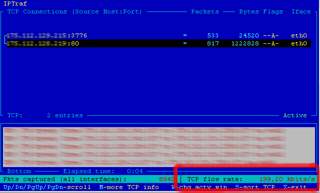
Et sur une autre machine, on lance un telnet vers le port 80 de la machine en écoute. L’outil iptraf permet de visualiser la connexion en cours et, surtout, son débit (voir figure 2).

figure2-debitqos

Comme on le voit dans l’encadré rouge, en bas à droite, le débit de la connexion est de 199,20kbps. On s’approche de beaucoup des 200kbps, la précision dépendant quelques paramètres que nous allons étudier. Si l’on teste une connexion du même type sur un autre port, on verra un débit limité à 1024kbps, ce qui correspond au débit de la classe par défaut qui s’applique à tous les paquets non marqués.

Lire la suite…